
What Compression Did to Your Data While You Slept
An engineer trends last night's pressure and sees a smooth line through the upset she knows happened. Nothing is broken and nothing was deleted. A compression deviation set to save disk in 2011 and a retrieval mode that paints straight lines through gaps did the rest.

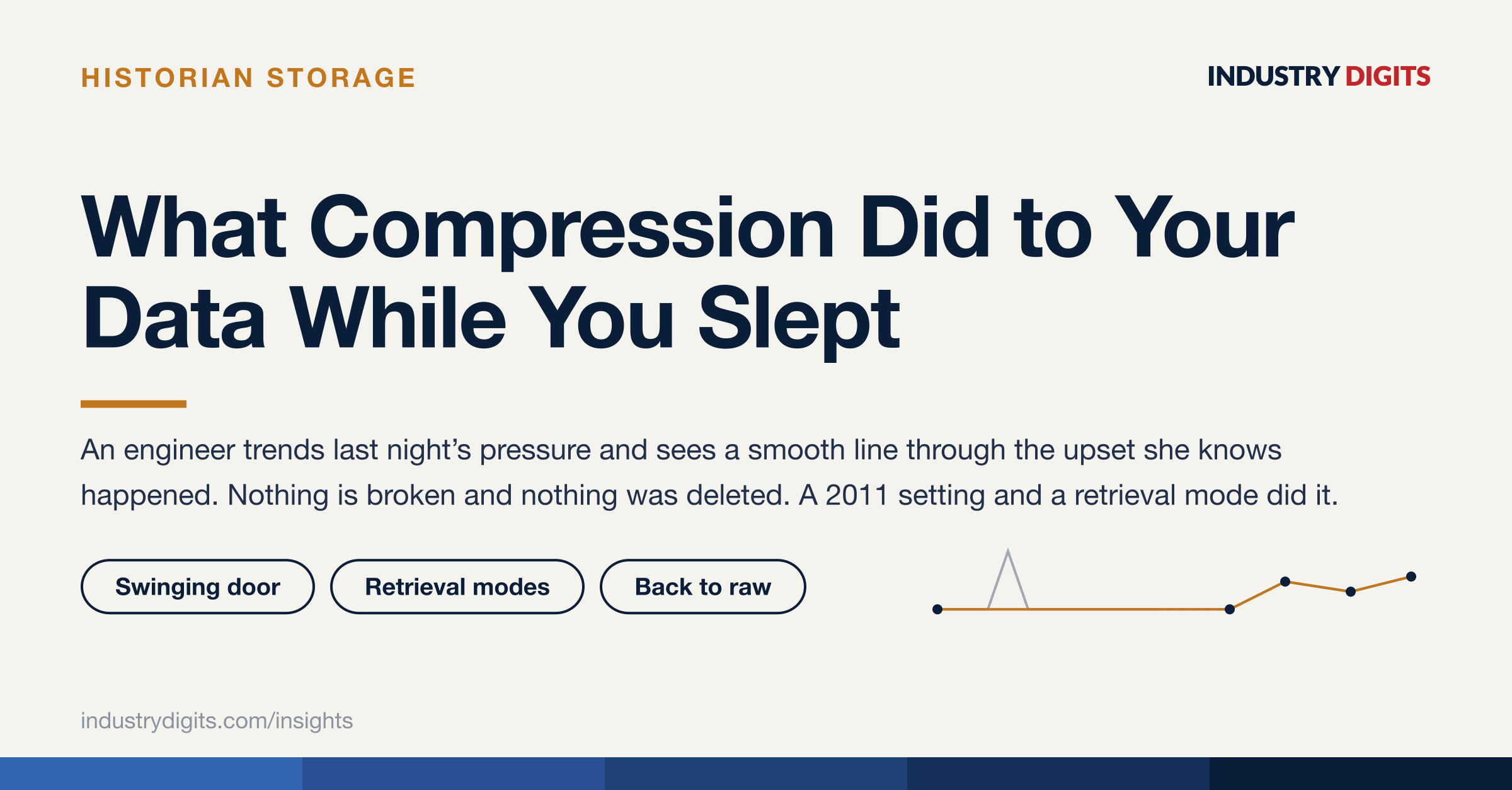
An engineer trends a pressure tag for last night and sees a smooth line through the upset she knows happened.
The historian is not broken. Nothing was deleted. Two mechanisms, both documented, both configured years ago, produced the picture.
Swinging-door compression kept only the points needed to reconstruct the signal within a configured deviation — and the deviation, set generously to save disk in 2011, was wider than the upset’s excursion. Then retrieval interpolated between the surviving points, drawing confident straight lines through the gap where the event used to be.
The record is exactly as specified. The specification just happened quietly, long ago, to data nobody had met yet.
Which is why compression settings are measurement decisions, not storage decisions.
Two families, one of which forgets on purpose
Lossless families. Modern open time-series engines lean on lossless per-series encodings — delta-of-delta timestamps, XOR-based value encoding, dictionary and run-length schemes. Slow-moving plant values compress spectacularly, because an unchanging value is almost free to store, and the record retrieved is bit-for-bit the record written.
If acquisition already deadbanded sensibly, lossless storage adds no new distortion. It is the honest default wherever the engine offers it.
Lossy families. The process-historian tradition adds deviation-based point selection: exception filters at ingest, and swinging-door trending — keep a point only when a new value cannot be reconstructed within a configured deviation by a straight line from the last kept point.
Ratios of ten to one beyond lossless are routine, and entire eras of plant history exist only because swinging-door made them affordable. That is not a small contribution and it should not be dismissed.
The price is the opening story. Excursions inside the deviation vanish. Small oscillations flatten. The lost detail is unrecoverable, and the setting is a permanent decision made per tag, usually by default.
The discipline mirrors the deadband exactly: derive the deviation from measured noise and named decision sensitivity, per tag class; record the setting in the point’s metadata; and re-examine it when a tag’s duty changes. The tag that fed a monthly report tolerates a deviation the same tag feeding a model cannot.
There is a question worth asking out loud, because storage economics have moved: is lossy compression still buying anything worth its epistemics? On modern hardware it frequently is not, and the setting persists because nobody has revisited it — which is a different thing from having chosen it.
Retrieval is the second half of the truth
What comes back from a query is not “the data”. It is a retrieval mode applied to the stored points, and consumers who do not know which mode they asked for get confidently misled.
| Retrieval mode | What it returns | Honest for | Lies when |
|---|---|---|---|
| Raw / actual | the stored points, as kept | investigations, model training, audit | you forget compression already thinned it |
| Interpolated | values computed on a regular grid between stored points | aligning tags for calculation and export | the signal was stepped, or the gap was an outage rather than a quiet period |
| Aggregates — avg, min, max, count | summaries per window | dashboards, KPIs, long-window trends | the consumer mistakes the average for the excursion; min and max discarded |
| Stepped / last-known | the value held until the next stored point | discrete states and report-by-exception data | applied to genuinely continuous signals |
Three rules keep consumers honest.
Match the mode to the signal’s semantics. Report-by-exception and discrete data are step functions and must be retrieved stepped. Interpolating them invents transitions that never happened, and the invention is invisible in the chart.
Distinguish “no data” from “no change”. An outage gap interpolated into a smooth line is the chain’s most dangerous lie, because it looks exactly like a calm period. Quality codes and gap markers exist so that retrieval can say unknown here — but the consumer has to ask, and most do not.
Investigate on raw. Trends and dashboards may live on aggregates and interpolation for speed. Any investigation, any model, and any argument with money attached goes back to the stored points — knowing that even “raw” is post-compression.
The audit that finds the erased events
The uncomfortable property of compression loss is that it leaves no trace. You cannot look at a trend and see what is missing, because the missing thing is precisely what was not stored.
There is one way to find out, and it only works forwards.
- 01 Pick a tag whose behaviour you know
Something with a documented event in recent memory — a trip, an upset, a batch transition somebody investigated. You need a known truth to compare against, because the archive alone cannot tell you what it forgot.
- 02 Retrieve it four ways
Pull the same window as raw, interpolated, an aggregate average, and stepped. Put the four on one page. The differences between them are the shape of what your consumers have been reading without knowing which mode they got.
- 03 Find the deviation setting and its derivation
The setting will exist. The derivation almost certainly will not. Record 'inherited default' honestly rather than reconstructing a justification — the absence is the finding, and it applies to every tag configured in the same pass.
- 04 Compare the excursion against the deviation
If the known event's excursion is smaller than the configured deviation, the archive cannot show it and never could. That is not a fault; it is a specification, and now it is a visible one.
The second step is the one that changes behaviour, because it converts an abstract warning into a picture. Four lines that disagree, drawn from the same tag over the same hour, tend to end the argument about whether retrieval mode is a real concern.
An exercise that costs an afternoon
Take the last incident anyone investigated with historian data — the one where the trends were used to build a timeline.
Re-run it on raw.
Then find out which mode the original investigation used. In most plants nobody recorded it, and in many the default was interpolated, which means the timeline was built partly from values that were computed rather than measured.
Two outcomes are common, and both are cheap to establish.
The picture is materially the same, which tells you compression and retrieval are not currently costing you anything on that class of tag — a genuinely useful result, worth writing down so the question stops recurring.
Or the picture is different, which tells you something more valuable: every conclusion drawn from that archive has a confidence attached that nobody has been stating. That does not invalidate the conclusions. It does mean the next investigation should start with a retrieval decision rather than a chart.
Neither outcome needs capital. Both change what the data contract for those tags should say.
Which of your trends could you prove was built from stored points rather than from painted ones?
The lossless and lossy mechanisms, the four retrieval modes, the three consumer rules, and the treatment of compression settings as measurement decisions are from Industrial IoT and Data Architecture: From Sensor to Historian to Dashboard (Part 4: Historians and Time-Series Storage, section 4.2).
Lokesh Chennuru writes Industry Digits field notes for industrial decision makers, focused on automation, IIoT, condition monitoring, predictive maintenance, and industrial AI.
Connect on LinkedInQuestions industrial leaders ask about this
What is swinging-door compression?
A deviation-based point-selection method used across process historians: a point is kept only when a new value cannot be reconstructed within a configured deviation by a straight line from the last kept point. It is highly effective — ratios well beyond lossless are routine — and it is lossy. Excursions smaller than the configured deviation vanish permanently, and small oscillations flatten.
Why is a compression setting a measurement decision rather than a storage decision?
Because it determines what the record can ever say. A deviation chosen for disk economy fixes, in advance, the smallest event the archive will be able to show — for data that had not been collected yet, feeding decisions nobody had proposed. The discipline is the same as for a deadband: derive it from measured noise and named decision sensitivity, record it in the point's metadata, and re-examine it when the tag's duty changes.
What are the retrieval modes and why do they matter?
Raw returns the stored points as kept. Interpolated computes values on a regular grid between stored points. Aggregates return summaries per window. Stepped holds the last value until the next stored point. What comes back from a query is a mode applied to stored points, not the data — and a consumer who does not know which mode they asked for is being confidently misled.
When does interpolation lie?
When the underlying signal was stepped rather than continuous, and when the gap was an outage rather than a quiet period. Interpolating report-by-exception or discrete data invents transitions that never happened. Interpolating across an outage paints a smooth line through a period where nothing was known, which is the chain's most dangerous single lie because it looks like data.
Should investigations use raw data?
Yes. Trends and dashboards may live on aggregates and interpolation for speed, but any investigation, any model training, and any argument with money attached goes back to the stored points — knowing that even raw is post-compression, which is the final reason the compression settings were measurement decisions all along.
Industrial IoT and Data Architecture — From Sensor to Historian to Dashboard
The nine-part reference this series draws on: the data value chain, the sensing layer, edge and acquisition, plant networks, historians and time-series storage, context and asset models, dashboards and analytics, security and chain reliability, and the implementation playbook — 40 sections covering signal families, protocol theories, timestamp discipline, compression and retrieval, tag naming, asset models, data contracts, notification engineering, threat modelling, and the pilot-to-wave economics a finance function can audit.