Remaining Useful Life: A Window, Not a Date

A model returns a number. RUL: 47 days.

Somebody puts it on a slide. By the time it reaches the outage meeting it has become a date — the twelfth of next month — and by the time it reaches the budget conversation it has acquired a confidence percentage nobody computed.

Two transformations happened between the fit and the meeting, and the data authorised neither of them. This article is about putting both back.

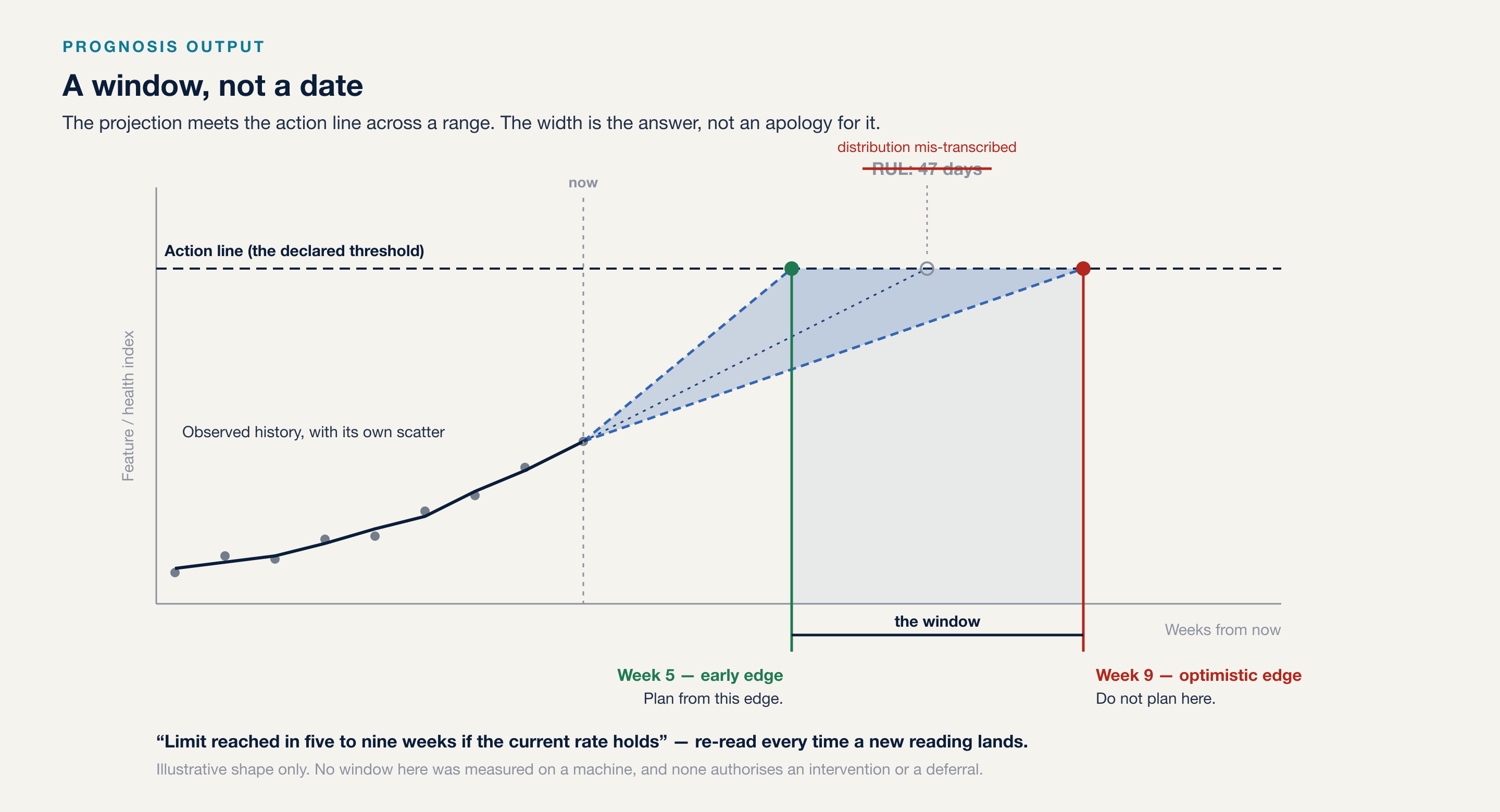
Prognosis is the summit of the analytics ladder and the most oversold rung in the market. It is also genuinely useful, provided it is quoted as what it is: a window, read from its early edge, re-read every time a new reading lands.

Most of your history is machines that did not fail

Start with the property that shapes everything downstream. A plant’s degradation histories are censored.

Most units in your records were repaired, replaced, moved to another duty, or are still running. What the data actually says about them is “lasted at least this long” — not “failed at this time”. The failures you have are the minority, and they are a self-selected minority: the ones that got that far without somebody intervening.

So a projection built from a censored, small, self-selected history is a planning input, not a forecast of when the machine will fail. It is consumed at its pessimistic edge, re-read as data arrives, and quoted as a range.

Anything that leaves a model as a date has had its distribution mis-transcribed somewhere between the fit and the meeting.

Three honest forms

There are three shapes a defensible prognosis takes, and each has an output discipline that travels with it.

Form	Mechanism	Fits when	Output discipline
Trend extrapolation to threshold	Project the feature or health index to the alarm line, carrying the trend’s own scatter forward	A single dominant degradation with a monotonic feature — the bearing and fouling staples	A window, never a date: “limit reached in five to nine weeks if the current rate holds”
Degradation-model regression	Fit the expected curve shape the physics implies — linear wear, exponential defect growth — and project with uncertainty	The mechanism is known from the failure-mode library, and the history is moderate	A window plus the model form you assumed, re-fitted as data arrives
Learned RUL	Match the current trajectory against fleets of run-to-threshold histories	Fleet-scale degradation archives exist, which on most plants they do not	As above, and no planning use until a claimed-versus-actual record exists for that asset class

Two of those cells deserve unpacking.

“If the current rate holds” is the assumption doing all the work. It is not a caveat appended to the sentence; it is the sentence’s load-bearing wall. Duty changes, a re-rate, a product change, a rebuild — each of them invalidates the extrapolation without moving the feature at all.

When each re-fit moves the window sharply, the model form is wrong, not the machine. That is a diagnostic worth writing down. A window that lurches every time it is recalculated is telling you the assumed curve shape does not match the degradation, and no amount of additional data will fix a mis-specified shape.

Read it from the early end

The uncertainty rule holds across all three forms, and the operational reason is the planner’s, not the statistician’s.

The planner consumes the pessimistic edge of the window against the response path — spares, crew, permits, outage slot. So a prognosis without a lower bound is unusable however good its centre. “About seven weeks” is not a planning input. “Five to nine weeks if the current rate holds, re-read fortnightly” is.

Two honesty requirements travel with the band.

Quote it for what it is. The band is the spread of a fit over a censored, small, self-selected history, widened by every assumption the fit needed. It is not the probability that the machine fails on a given day. Dressing it as one — “act-by date, 90% confidence” — lends a regression the authority of an actuarial table it has not earned.

Read it from the early end. The asymmetry here is the planner’s own: late costs catastrophically and early costs linearly. The field learned this in public. In 2008 the young prognostics and health management community staged its first open data challenge on NASA’s C-MAPSS turbofan simulations, scored by a penalty that punished late predictions more harshly than early ones. What that record supports is narrow and worth stating exactly: that the field priced lateness more heavily than earliness, on simulated turbofan data. It does not transfer a score, a method ranking, or a scoring function to your assets. Your own consequence arithmetic sets that.

ISO 13381-1 puts the same maturity institutionally, and is worth naming so a reader can find it: it orders the prognostic process so that prognosis is the final step, after detection, diagnosis and degradation assessment, with the confidence in each step carried forward. Naming it is orientation, not a conformity claim.

A fleet hazard is not a prediction about your machine

Trajectory prognosis needs a degradation curve to ride. Many assets offer none — the random-pattern population that no trend method can touch. For those, the honest move is to change the question from the machine to the fleet.

Survival analysis was built for exactly this data. Kaplan and Meier (1958) solved estimating survival curves when most subjects have not died yet. Cox (1972) showed how risk factors scale a hazard without needing its full shape. Weibull’s earlier distribution work supplies the shape parameter. A plant’s asset fleet is a survival study: a handful of failures, a majority of survivors still running, and covariates — duty, environment, rebuild history — begging to be tested.

But the answers are fleet-sized. A fleet hazard of three per cent a year is not a three per cent chance for your gearbox. It is a statement about a population your gearbox happens to belong to, whose members differ from it in every way the model never recorded.

And the parameters need their intervals quoted or they should not be quoted at all. For a complete sample, the standard error of ln β̂ is roughly 0.78/√r, where r is the number of observed failures. Censoring widens it further.

Work it through on the reference’s illustrative composite site. Meridian’s gearbox fleet returned β̂ ≈ 0.9 on six observed failures. So exp(±1.96 × 0.78/√6) puts the 95% interval at roughly 0.5 to 1.7 — and because the fleet’s survivors are censored, that is the narrowest the interval can honestly be.

The point estimate leans just below one. The range rules out none of infant mortality, constant hazard, or mild wear-out. The honest reading is therefore not “random-dominated, confirmed”. It is that six failures cannot separate those three patterns, so a calendar overhaul interval on this fleet has no support in the data. That is a weaker statement than saying the data refutes the interval, and a far more defensible one.

Deferral is where prognosis does most of its damage. A window that reads “at least six more weeks” is the easiest thing in the plant to quote and the hardest thing to defend afterwards.

An exercise that costs an afternoon

Find the last five prognosis windows your programme issued. Any five.

For each one, write down two things on the same line: what the window said before the machine was opened, and what was actually found when it was. Not the outcome — the as-found stage, in the same vocabulary the window used.

Most teams cannot complete more than one or two lines, and the reason is almost never that the models were bad. It is that nobody kept the claim. The window was quoted in a meeting, the job was done, and the pair was never closed.

That missing pair is the whole difference between a prognosis that is an opinion and one that is an instrument. It is also free to start collecting, from the next window you issue, using nothing but a column in a spreadsheet you already own — and it is worth keeping most carefully in exactly the cases where the window turned out to be badly wrong.

What did your last remaining-useful-life estimate say before the machine was opened, and can you still find it?

The three prognosis forms, the censoring rule and the shape-parameter interval arithmetic above are from Predictive Maintenance: Practitioner Reference Frameworks and Planning Guide (Part 9: Analytics, AI, and Prediction Models).