450-Minute Shift: How OEE Boundaries Hide Real Losses

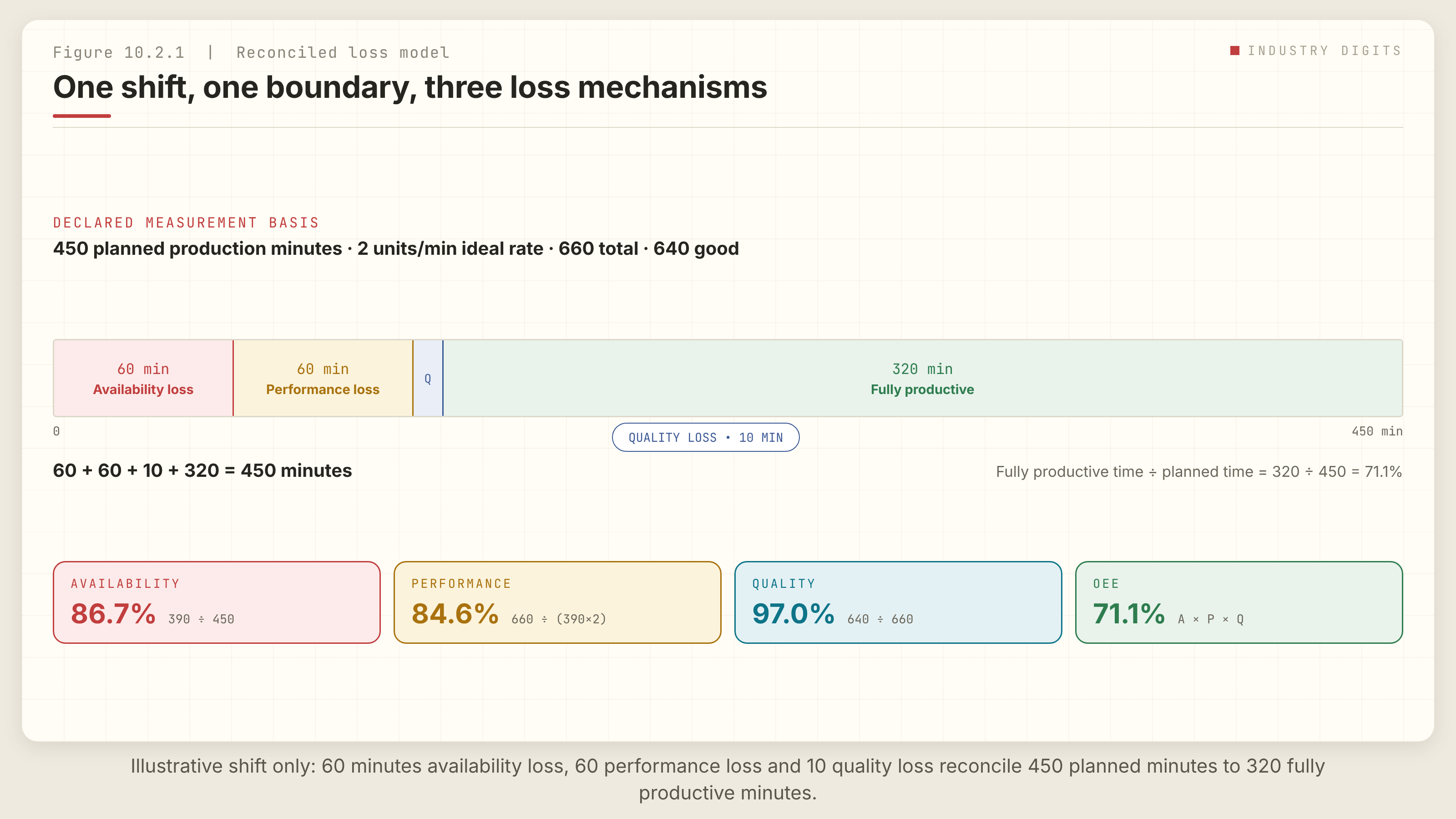
Here is one shift, reconciled to the minute.

A line is planned to produce for 450 minutes at an ideal rate of 2 units per minute. It actually runs 390 of those minutes; 60 are lost to stops. In its running time it makes 660 units where the ideal rate says 780. Of the 660 made, 640 are good.

Every planned minute lands in exactly one category:

Category	Minutes	Where it comes from
Availability loss	60	450 planned − 390 actually running
Performance loss	60	120 missing units ÷ 2 per minute
Quality loss	10	20 rejects ÷ 2 per minute
Fully productive	320	what’s left
Planned total	450

And the three factors:

Factor	Calculation	Result
Availability	390 / 450	86.7%
Performance	660 / (390 × 2)	84.6%
Quality	640 / 660	97.0%
OEE	86.7% × 84.6% × 97.0%	71.1%
Check	320 / 450	71.1%

The two routes agree, because they are the same statement made twice. That is the whole point of the reconciliation: if your loss categories don’t add back to planned time, one of them is absorbing something nobody has named.

The arithmetic takes five minutes. Everything hard about OEE is in what the arithmetic sits on.

The number is honest; the boundary decides

OEE locates losses inside a declared boundary. Change the boundary and the number moves without the plant changing at all.

Reclassify a changeover from downtime to planned exclusion, and availability improves on paper. Nudge the ideal cycle time from what the machine proved to what the budget assumed, and performance improves on paper. Count rework as good on first pass, and quality improves on paper.

None of these makes a single extra unit.

Planned time is where most of it happens. It is the least examined of the three inputs and the easiest to move, because moving it rarely feels like cheating. Somebody decides that planned maintenance shouldn’t count against the line. Then changeovers, because they’re scheduled. Then the daily start-up sequence, because it’s unavoidable. Then the meeting. Each exclusion is individually defensible and the aggregate is a line that reports 85% while producing for two thirds of the time it was staffed.

The test isn’t whether an exclusion is justifiable. It’s whether the excluded time is genuinely unavailable for production or merely currently consumed by something else. Changeover time is not unavailable. It’s a loss you have decided to stop counting, and SMED programs exist precisely because it is recoverable.

Ideal rate is the second lever. There are three candidate numbers — nameplate, best demonstrated, and budget assumption — and they are rarely equal. Whichever you pick, write down which one it is and why. A performance factor computed against an ideal rate the machine has never achieved measures the ambition of the last capital request.

This is also why comparing OEE across lines or plants with different boundaries mostly measures the boundaries. Two sites reporting 78% may be running very differently. Two sites running identically may report 78% and 64%.

Used honestly, though, the three-factor split earns its reputation. It answers, in one line: is the line on, is it fast, is it good? Those are three different problems, owned by different people, fixed by different work — and separating them is worth more than the composite score ever is.

What OEE cannot tell you

The reconciliation locates the loss. It does not explain it.

Sixty minutes of availability loss might be one breakdown or twelve short stops. Identical in the score; completely different in the fix — and the twelve short stops are usually the more expensive problem, because nobody raises a work order for a two-minute jam.

The performance factor can hide slow-and-steady degradation that never trips an alarm and never appears in an event log. A line running at 92% of rate for six months loses more than a line that stops hard for a day, and only one of them gets a meeting.

And OEE says nothing about whether the lost minutes were worth recovering. Capacity a market doesn’t want is an exercise, not an improvement. A line at 71% that meets demand comfortably may be exactly where it should be; the question is what the next constrained period looks like, not what the dashboard says today.

So treat the score as a pointer into the evidence, not a verdict: from the loss category to the event log, from the event log to causes, from causes to the one bounded change worth testing.

An exercise that recalibrates a team

Reconcile one shift by hand, the way the tables above do it. Planned time, availability loss, performance loss, quality loss, in minutes, until the total closes to the planned figure.

Use the line’s own raw data — not the dashboard’s summary, which is the thing under examination.

Two things reliably happen. Somebody discovers the dashboard’s boundary decisions, usually inside the planned category, and the room gets briefly quiet. And the category that surprises you shows where measurement, rather than the plant, was doing the lying.

A 71.1% shift, honestly measured, is a better starting point than an 85% shift with a flattering boundary. Only one of them can be improved.

What’s excluded from planned time on your line — and who decided?

The worked shift above, the reconciled-loss figure, and the boundary checklist are from Industrial Automation: Real-World Frameworks & Implementation Guide (Part 10: operations and optimization).